Data Analytics – Text Mining the 2006 AOL Web Search Logs

Data Analytics – Text Mining the AOL 2006 Web Search Logs

By Kato Mivule

• In this example, we use R to implement text mining of the 2006 AOL web search logs.
• The 2006 AOL data set is multivariate – containing more than one variable.
• In this example, we are interested in the Query variable – containing the actual queries that were issued by users.

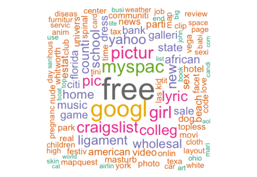
The 2006 AOL Web Search Logs WordCloud Sample

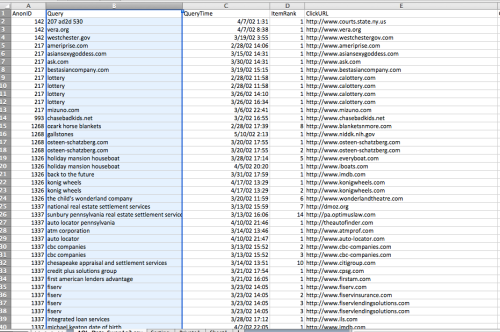
The AOL Dataset

• The AOL dataset published by AOL in 2006, is one of the few public datasets available that contain real web search logs.

• While data curators at AOL claimed to have “anonymized” the dataset by removing personal identifiable information (PII), researchers were able to re-identify some individuals in the published dataset.

• The AOL dataset contains the following five variables (attributes):
  • AnonID: stores the identification number of the user.
  • Query: stores the actual query that the user executed.
  • QueryTime: The date and time the query was executed.
  • ItemRank: AOL’s ranking of the query.
  • ClickURL: The actual URL link that the user clicked on after querying.

Big Data Analytics

• The big data problem then becomes apparent; we are looking at about 1.5 gigabytes of data.

• There are about 20 Million web queries collected from about 650, 000 individuals over a 3 month period.

• However, I have only labeled a sample of about 500 Megabytes of data for machine learning purposes. We could use this sample as a start.

In this case we use R Studio for the implementation.

You can download R Studio here… https://www.rstudio.com/

You can download the 2006 AOL web search logs here… http://www.gregsadetsky.com/aol-data/

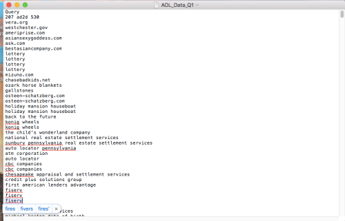
Step 1 – Select the Query attribute for analysis.

• We are interested in doing text-mining analytics on the actual queries that were issued by the users.
• In this example, we only use about 55,000 rows of data (queries) from the Query attribute – about 1.8 megabytes of data for our text analytics.

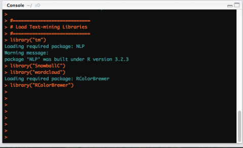
Step 2 – Load the text-mining libraries in R

• In this case, we use the “tm” library for text-mining.

library("tm")

library("SnowballC")

library("wordcloud")

library("RColorBrewer")

Step 3 – Read/input the text file containing the query data into R Studio.

filePath1 <- "~/Desktop/AOL_QUERY_PRIVACY1/AOL_Data_Q1.txt"

• In this example, we use about 50,000 rows of text data, about 1.8 megabytes.

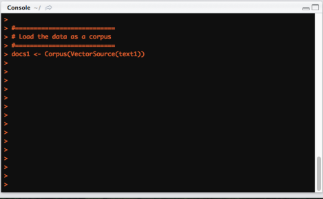
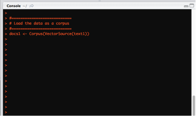
Step 4 – Load the data into a corpus

• Text is transformed in a corpus, which is a set of documents. In this case, each row of data in the query variable (attribute) becomes a document.

docs1 <- Corpus(VectorSource(text1))

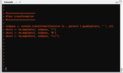
Step 5 – Do a Text Transformation

• Replace special characters,“/”, “@”, “|” , etc, with space.
• The tm_map() function is used to replace special characters in the text.

toSpace <- content_transformer(function (x , pattern ) 
gsub(pattern, " ", x))

docs1 <- tm_map(docs1, toSpace, "/")

docs1 <- tm_map(docs1, toSpace, "@")

docs1 <- tm_map(docs1, toSpace, "\\|")

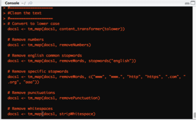
Step 6 – Transform and clean the text of any unnecessary characters.

# Transform text to lower case

docs1 <- tm_map(docs1, content_transformer(tolower))

# Transform text by removing numbers

docs1 <- tm_map(docs1, removeNumbers)

# Transform text by removing english common stopwords

docs1 <- tm_map(docs1, removeWords, stopwords("english"))

Transform text by removing specific stopwords. These words tend to be very common in the AOL Web search logs and offer no meaning at this point, but are a distraction in the analytics by giving us unneeded stats – “www”, “www.”, “http”, “https”, “.com”, “.org”, “aaa”.

docs1 <- tm_map(docs1, removeWords, c(“www”, “www.”, “http”, “https”, 
“.com”, “.org”, “aaa”))

# Transform text by removing punctuations

docs1 <- tm_map(docs1, removePunctuation)

# Transform text by removing whitespaces

docs1 <- tm_map(docs1, stripWhitespace)

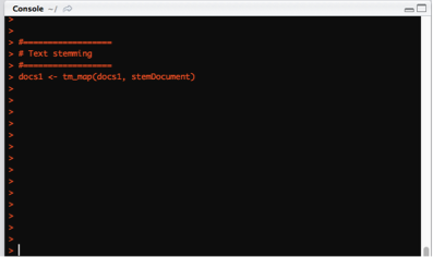
Step 6 – Transform by Text Stemming – reducing English words to their root.

• In this step, English words are transformed and reduced to their root word, for example, the word “running” is stemmed to “run”.

docs1 <- tm_map(docs1, stemDocument)

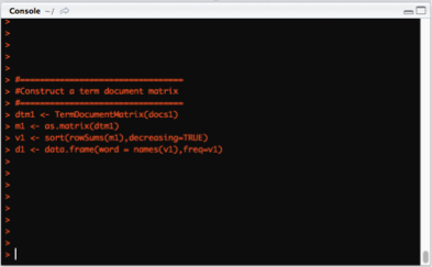
Step 7 – Construct a document matrix.

• A document matrix is a table made up of each unique word in the text and how many times it appears – basically the table of word frequency.
• The column names in the table are each unique word and row names represent the documents in which those words appear.
• The TermDocumentMatrix() function from the “tm” library is used to generate the document matrix.
• The document matrix is what we use for the frequency analytics of words in the text to finally derive conclusions.
• The matrix() function transforms the TermDocumentMatrix into a matrix.
• The sort () function transforms text by sorting it in descending or ascending order.
• The frame () function creates is a list of variables of the same number of rows with unique row names, given class “data.frame“, in this case we create variables of words and their frequencies.
• The head () function returns the top 10 most frequent words in the data.frame, d1.

dtm1 <- TermDocumentMatrix(docs1)

m1 <- as.matrix(dtm1)

v1 <- sort(rowSums(m1),decreasing=TRUE)

d1 <- data.frame(word = names(v1),freq=v1)

head(d1, 10)

Step 8 – Do a frequency analysis

• At this point we can take a look at the most frequent terms, or in this case queries issued.
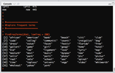
• The findFreqTerms() function is used to find the frequent terms or words used in the term-document matrix.
• In this case, we want to get words at appear at least 200 times.

findFreqTerms(dtm1, lowfreq = 200)

Results from the head () function

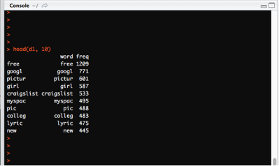
Words that appear at least 200 times.

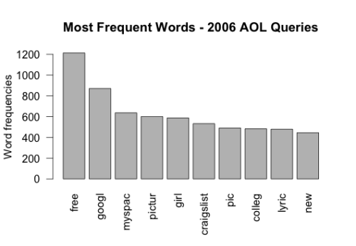
Step 9 – Plot the word frequencies

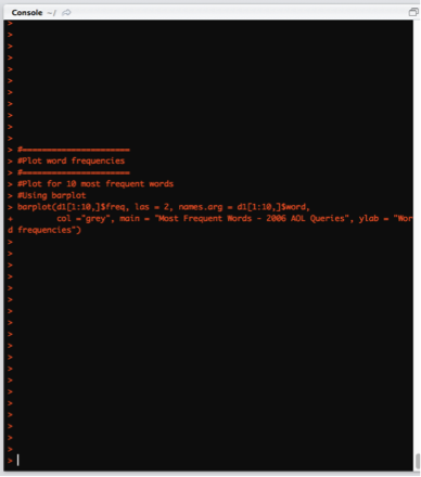
• The barplot () function is used to plot the 10 most frequent words from the 2006 AOL sample we used.

barplot(d1[1:10,]$freq, las = 2, names.arg = d1[1:10,]$word, col =“grey”, 
main = "Most frequent words", ylab = "Word frequencies")

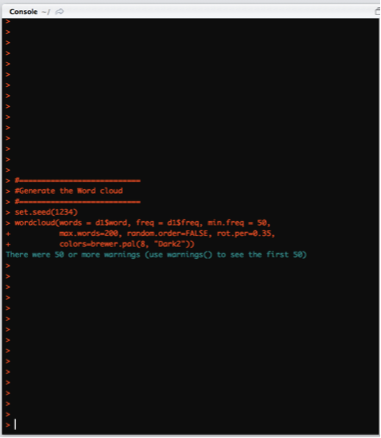
Step 10 – Generate a word cloud of words that appear at least 200 times.

• The wordcloud () function from the wordcloud library is used to plot the word cloud for the queries under analysis.
• The words parameter in the wordcloud represents the words to be plotted.
• The freq parameter represents the word frequencies.
• The freq parameter sets a limit on words with a certain frequency to be plotted.
• The words parameter sets the maximum number of words to be plotted.
• The order parameter plots words in random order. If set to false, words will be will be plotted in decreasing frequency.
• The per parameter vertically proportions words with a 90-degree rotation.
• The colors parameter sets the color of words from the least to most frequent.

set.seed(1234)

wordcloud(words = d1$word, freq = d1$freq, min.freq = 50, max.words=200, 
random.order=FALSE, rot.per=0.35,colors=brewer.pal(8, "Dark2"))

The word cloud.

Conclusion

From this data sample, we can conclude that terms such as “Google”, “Yahoo”, “Free”, “Myspace”,”craigslist”, were popular search terms then on the AOL search engine in 2006.

References

1. Michael Arrington, “AOL Proudly Releases Massive Amounts of Private Data”, TechCrunch, Accessed Feb 17 2016, Available Online at: http://techcrunch.com/2006/08/06/aol-proudly-releases-massive-amounts-of-user-search-data/

2. Michael Barbaro and Tom Zeller, “A Face Is Exposed for AOL Searcher No. 4417749”, New York Times, Accessed Feb 17 2016, Available Online at: http://www.nytimes.com/2006/08/09/technology/09aol.html

3. Greg Sadetsky, “AOL Dataset”, Accessed Feb 17 2016, Available Online at: http://www.gregsadetsky.com/aol-data/

4. com – Text-mining and Word Clouds – http://www.sthda.com/english/wiki/text-mining-and-word-cloud-fundamentals-in-r-5-simple-steps-you-should-know

 

 

 

 

 

Data Analytics Simplified – A Tutorial – Part 6 – Data Analytics Challenges

Data Analytics Challenges

By Kato Mivule

Part 1, Part 2, Part 3, Part 4, Part 5

There are a number of challenges any data analytics project will have to give serious consideration. Below, we identify and classify five main challenges that any data analytics specialist will always encounter: (i) the problem definition challenge, (ii) the data preprocessing challenge, (iii) the big data challenge, (iv) the unstructured data challenge, and (v) the evaluation of results challenge [1] [2] [3] [4].

The problem definition challenge

• Many data analytics problems are not well defined by stakeholders and therefore require a collaboration between domain and technical specialists to determine the data to be used and outcomes, and the algorithms needed to accomplish the tasks.

The data preprocessing challenge

• Most of the datasets presented for data analytics comes incomplete and not in the required format to properly apply data analytics algorithms. During the data preprocessing stage, data has to be placed in a format suitable for the data mining and machine learning algorithms.
  • Missing values: during the preprocessing phase, missing values in the data have to be replaced with average values or the most frequent values.
  • Noisy data: incorrect and invalid values have to be removed and replaced as well.
  • Irrelevant values: values that offer no insight to the problem being solved are removed at this stage.
  • Outliers: these are values that are too high or too low that they affect the overall outcome of the data analytics results. For example, a dataset containing the salary of both the CEO and Janitor might not reflect well on the average salary of workers in that organization. Yet simply removing the outliers would be a loss of valuable data, and therefore a challenge to data analytics.

The big data challenge

• The exponential growth of data on a daily basis presents an ever growing challenge for data analytics in terms of computation resources needed to analyze such datasets.
• The big data problem includes both the large datasets and the high dimensionality of such data sets, i.e., the large number of attributes or variables in a given dataset.

The unstructured data challenge

• Traditional data analytics always worked with structured data in well defined data structures such as, text, numeric, and date. However, of recent, due to the exponential growth and use of the internet, data is directly stored to data warehouses in unstructured formats that include multimedia formats such as images, video, GIS data, etc.
• Therefore unstructured data is a challenge for data analytics in that it has to be preprocessed to the right format before the analytics process.

The evaluation of results challenge

• Another challenge related to the problem definition challenge in data analytics is the evaluation of results. In both cases the user or stakeholders do not state precisely what they want to analyze and even when results are presented, it becomes a challenge to both the technical experts in interpreting and visualizing the results in a meaningful way to the stakeholders.
  • Result interpretation: Results that may be correctly interpreted by the data analytics specialists might sound meaningless to clients.
  • Result visualization: large datasets always present a visualization challenge, therefore the data analytics specialists are faced with presenting results in a succinct, understandable, and meaningful way to the users.
• The data analytics specialist has to find the balance between presenting too much and too little information.

References

[1] Margaret H. Dunham, “Data Mining: Introductory and Advanced Topics”, Prentice Hall, 2003, Page 9-10.

[2] David Boulton and Martyn Hammersley, “Analysis of unstructured data”, Chapter 10, Data Collection and Analysis, Editors: Roger Sapsford, Victor Jupp, SAGE, 2006, ISBN: 9780761943631, Page 243.

[3] Nathalie Japkowicz, Jerzy Stefanowski, “Big Data Analysis: New Algorithms for a New Society”, Volume 16 of Studies in Big Data, Springer, 2015, ISBN: 9783319269894, Pages 4-10.

[4] Jiawei Han, Jian Pei, Micheline Kamber, “Data Mining, Southeast Asia Edition”, The Morgan Kaufmann Series in Data Management Systems, Morgan Kaufmann, 2006,ISBN: 9780080475585, Page 47.

Data Analytics Simplified – A Tutorial – Part 5 – The Data Analytics Process

Data Analytics Simplified – A Tutorial – Part 5 – The Data Analytics Process

By Kato Mivule

Part 1, Part 2, Part 3, Part 4

The Data Analytics Knowledge Discovery Process

The data analytics process involves using algorithms to extract, mine, and discover meaningful information patterns and knowledge in data [1].

However, the data would have to undergo a series of transformational processes before meaningful information patterns can be extracted.

There are five main phases in the data analytics process [1] [2] [3] [4] [5]:

Problem formulation

• The first step of the data analytics process is to articulate the problem and questions that need to be solved and answered by the data analytics process.

• The question or problem to be solved has to be domain specific.

• This helps with the correct data selection process. For example local grocery stores might want to use traffic pattern data to predict when customers with cars are most likely to stop my a certain store.

Data Selection

• The second step of the process is to select an appropriate dataset based on a specific domain.

Data Preprocessing

• The third step is to transform the selected dataset into a format that could most appropriate for analytics algorithms.

• This process is also called data cleaning, in which missing values are removed or replaced with averages. Data outliers maybe removed or replaced with appropriate values. Data with different data types are also corrected at this stage.

• Data analytics work involves a considerable time preprocessing data to ensure correct analysis.

Data Transformation

• Data from different sources is then converted into a common format for analysis.

• This could include reducing the data into appropriate sample sizes, adding labels for classification and changing file types to make the data suitable for analytics tools.

Data Mining

• In this phase, appropriate data mining and machine learning algorithms are chosen.

• The analyst then could make a choice to employ supervised or unsupervised learning algorithms.

• In some cases, depending on the problem formulation, both supervised and unsupervised learning algorithms will be chosen.

• However, parsimony is important – keep it simple. You don’t need to implement all algorithms to extract meaningful knowledge from the data and come up with a correct model.

Evaluation

• In this phase evaluation of results produced by the data mining algorithms is done.

• The extracted knowledge is then presented to the stakeholders in a clear manner.

• Visualization of results is done at this stage.

• A report analyzing and interpreting the results to convey meaning is done at this stage.

• Again parsimony is important. A concise and understandable visualization of results is preferred.

References

[1] Margaret H. Dunham, “Data Mining: Introductory and Advanced Topics”, Prentice Hall, 2003, Page 9-10.

[2] Fayyad, Usama, Gregory Piatetsky-Shapiro, and Padhraic Smyth. “The KDD process for extracting useful knowledge from volumes of data.” Communications of the ACM 39, no. 11 (1996): 27-34.

[3] Dhar, Vasant. “Data science and prediction.” Communications of the ACM 56, no. 12 (2013): 64-73.

[4] Panov, Panče, Larisa Soldatova, and Sašo Džeroski. “OntoDM-KDD: ontology for representing the knowledge discovery process.” In Discovery Science, pp. 126-140. Springer Berlin Heidelberg, 2013.

[5] Sacha, Dominik, Andreas Stoffel, Florian Stoffel, Bum Chul Kwon, Geoffrey Ellis, and Daniel A. Keim. “Knowledge generation model for visual analytics.” Visualization and Computer Graphics, IEEE Transactions on 20, no. 12 (2014): 1604-1613.

Data Analytics Simplified – A Tutorial – Part 4 – Statistics

Data Analytics Simplified – A Tutorial – Part 4 – Statistics

By Kato Mivule

Part 1, Part 2, Part 3

Basic Statistics

The Normal Distribution – Credit: Wikipedia

• Data analytics is based largely on statistics and statistical modeling. However, a basic knowledge of descriptive and inference statistics should suffice for beginners.

Descriptive statistics

• Descriptive statistics are values used to summarize the characteristics of the data being studied. Such descriptions could include, values such as, the mean, maximum, minimum, mode, and median traits of values in a variable [1]. For example, we could say that for the following variable Y with values {2, 4, 3, 5, 7}, the maximum values is 7, while the minimum value is 2.

Inference statistics

• Inference statistics are used to infer and make conclusions about what the data being studied means. In other words, inference statistics is an attempt to deduce the meaning of the data and its descriptive statistics [2]. For this tutorial, we shall look at covariance and correlation as part of the inference statistics. While some data scientists spend time dissecting inference statistics in efforts to design new machine learning algorithms, in this tutorial, we are concerned with using data analytics as a tool to extract knowledge, wisdom, and meaning from the data. So, we shall focus on the application side rather than on the design side of data science. In other words, we shall be looking at how to apply data science algorithms to solve data analytics problems and leave the design of such algorithms for the advanced stage. Therefore, basic statistics such as, normal distribution, mean, variance, standard deviation, covariance, and correlation will be given consideration.

Descriptive statistics

• Mean

The Mean μ, is the average of numeric values after the total of those values has been computed. The summation (total) of the values, symbolized by is taken and then divided by the n, the number of values as show in the following formula [3]:

• Mode

The mode is the value or item that appears most – the frequent, in an attribute or dataset [4].

• Median

The median represents the value that separates a data sample into two parts halves – the first half from the second half [4].

• Minimum

The minimum is the smallest value in a variable or dataset [5].

• Maximum

The maximum is the largest value in a dataset or variable [5].

• Range

The range is the measure of dispersion and spread of values between the minimum and maximum in a variable [6]. 

• Frequency Analysis

A frequency analysis is a count of times items or values that appear in a data sample. The frequency metric can be described using the following formula [7]:

Where items(c) is the set of items in a dataset c.

• Normal Distribution

The Normal Distribution N (μ, σ²), (Gaussian distribution), is a bell shaped continuous probability distribution used as an estimation to show how values are spread around the mean value. The normal distribution can be computed as follows [3]:

The parameter μ represents the mean, the point of the peak in the bell curve. The parameter σ² symbolizes the variance, which is the width of the distribution. The annotation N (μ, σ²) represents a normal distribution with mean μ and variance σ². Therefore X is descriptive of the normal distribution of the variable X between N (μ, σ²). The distribution with μ = 0 and σ 2 = 1 is known as the standard normal.

• Variance

The Variance σ², is a calculation of how data distributes itself in approximation to the mean value. Variance can be calculated as follows [3]:

Where the symbol σ² is the variance. The symbol µ is the mean. The symbol X is the data values in the variable X. The symbol N is the total number of values. The symbol ∑ (X – µ)² is the summation of all data values in the variable X, minus the mean µ.

• Standard Deviation

The Standard Deviation σ, calculates how data values deviate from the mean, and can be computed by simply taking the square root of the variance σ² as follows [3]:

 

Inference statistics

• Covariance

Covariance Cov (X, Y), is a calculation of how associated the deviations between the data points X and Y are [3]. If the covariance is positive, then data values increase together, else if negative, then for the two data points X and Y, one diminishes while the other increases. If the covariance is zero, then this shows that the data values are each independent. Covariance can be calculated as follows [3]:

Correlation

• Correlation calculates the incline of a linear relation between two data points x and y [3]. The correlation is independent of the parts in which the data points x and y are calculated. The correlation values are measured between 0 and 1. However, if the correlation is negative (-1) the linear relationship between the two data points is negative. If the correlation is 0, then the linear relationship between the two data points is non-existent. If the correlation approaches the value of 1, then the linear relationship is exists and gets stronger as the correlation values approaches 1. Correlation can be computed using the following formula [3]:

References

[1] Wikipedia, “Descriptive statistics”, Accessed 02/26/2016, Available Online: https://en.wikipedia.org/wiki/Descriptive_statistics

[2] Wikipedia, “Statistical inference”, Accessed 02/26/2016, Available Online: https://en.wikipedia.org/wiki/Statistical_inference

[3] Kato Mivule, “Utilizing Noise Addition for Data Privacy , an Overview.” In Proceedings of the International Conference on Information and Knowledge Engineering (IKE 2012), 2012, Page 65–71.

[4] Larry Hatcher, “Step-by-Step Basic Statistics Using SAS: Student Guide”, SAS Institute, 2003, ISBN 9781590471487, Page 183

[5] Dennis Cox and Michael Cox, “The Mathematics of Banking and Finance”, John Wiley & Sons, 2006, ISBN 9780470028889, Page 37

[6] Jacinta M. Gau, “Statistics for Criminology and Criminal Justice”, SAGE Publications, 2015, ISBN 9781483378442, Page 98.

[7] Philip Resnik. 1999. Semantic similarity in a taxonomy: An information-based measure and its application to problems of ambiguity in natural language. J. Arti cial Intell. Res. 11 (1999), 95–130.

Data Analytics Simplified – A Tutorial – 3

Data Analytics Simplified – A Tutorial – Part 3 

By Kato Mivule

Keywords: Supervised Learning, Unsupervised Learning

Part 1, Part 2

Data analytics can be broken down into two main categories as we saw in the previous post, predictive and descriptive data analytics. Furthermore, data analytics tasks can be categorized as follows:

Supervised learning tasks: This involves algorithms that group data into classes and make predictions based on previous examples – thus learning by example [1]. In other words data is grouped into predetermined classes based on previous history of categorizing the data. The data in supervised learning is always labeled (classes) and basically divided into:

• Training data – which is used for setting up examples on how to group the data, and thus create a model for future grouping of the data.
• Testing data – which is used to make predictions, based on the example data.

Unsupervised learning tasks: This involves algorithms that do not need predetermined classes to categorize the data [2]. In such cases, the data self determines the groups or clusters into which similar data values collect together.

• Predictive data analytics methods are largely supervised learning methods.
• Descriptive data analytics methods are mainly non-supervised learning methods.

 

Data Analytics – Supervised and Unsupervised Learning Tasks

Briefly, predictive data analytics includes the following three main data analytics methods, more details shall follow later:

• Classification analysis

Classification involves grouping or prediction of data into predefined categorical classes or targets. The classes in which the data is grouped are chosen before analyzing the data based on the characteristics of the data [3].

• Regression analysis

Regression involves the prediction or grouping of data items into predefined numerical classes or targets based on a known mathematical function such as a linear or logistic regression function [4].

• Time series analysis

Time series analytics involves examining the values of a data attribute that have been recorded over a period of time, in a chronological order. Predictions are made based on the history of the values observed over time [5] [6].

Descriptive data analytics includes the following unsupervised data analytics methods, more details shall follow later:

• Clustering

Clustering involves grouping data into classes but without any predefined or predetermined classes and targets. The classes in which the data is grouped are self-determined by the data, such that similar items collect around the same clusters [7].

• Summarization

Summarization is the generalization of data into groups that are related with descriptive statistics such as the mean, mode, and median [8].

• Association Rules

Associative rules involve using a set of IF-THEN rules or functions to categorize data with similar relationships in the same groups [9].

• Sequence Discovery

Similar to time series analysis, sequential discovery or sequential pattern analysis, involves finding the related patterns in sequential data – that is data in chronological order, based on statistical properties [10].

References

[1] Olivier Pietquin, “A Framework for Unsupervised Learning of Dialogue Strategies”, Presses univ. de Louvain, 2004, ISBN 9782930344638, Page 179.

[2] Nick Pentreath, “Machine Learning with Spark”, Packt Publishing Ltd, 2015, ISBN 9781783288526, Page 197.

[3] Ashish Gupta, “Learning Apache Mahout Classification Community experience distilled”, Packt Publishing Ltd, 2015, ISBN 9781783554966, Page 14.

[4] Robin Nunkesser, “Algorithms for Regression and Classification: Robust Regression and Genetic Association Studies”, BoD – Books on Demand, 2009, ISBN 9783837096040, Page 4.

[5] Gebhard Kirchgässner, Jürgen Wolters, Uwe Hassler, “Introduction to Modern Time Series Analysis”, Springer Texts in Business and Economics, Edition    2, illustrated, Springer Science & Business Media, 2012, ISBN 9783642334368, Page 1.

[6] George E. P. Box, Gwilym M. Jenkins, Gregory C. Reinsel, Greta M. Ljung, “Time Series Analysis: Forecasting and Control”, Wiley Series in Probability and Statistics, Edition 5, John Wiley & Sons, 2015, ISBN 9781118674925, Page 1.

[7] Brett Lantz, “Machine Learning with R”, Edition 2, Packt Publishing Ltd, 2015,ISBN 9781784394523, Page 286.

[8] Margaret H. Dunham, “Data Mining: Introductory and Advanced Topics”, Prentice Hall, 2003, Page 8.

[9] Norbert M. Seel, “Encyclopedia of the Sciences of Learning”, Springer Science & Business Media, 2011, ISBN 9781441914279, Page 2910.

[10] Wikipedia, “Sequential Pattern Mining”, Wikipedia, Accessed, February 15, 2016, https://en.wikipedia.org/wiki/Sequential_pattern_mining